TensorFlow Validation, Regularization, and Callbacks

Github Link

https://github.com/Natan-Asrat/tensorflow_validation_regularisation_and_callbacks

Contact

The Setup

Description

In this project i regularized a model using L2 regularization with dropout while also comparing the perfomance improvements visually by plotting loss during training and validation.

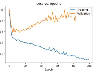
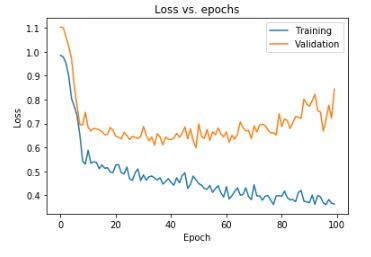
Due to reduced overfitting, the validation loss is decreased after using L2 regularization and dropout relative to the unregularized model.

Libraries Used

TensorFlow Keras
Matplotlib
Sklearn

Imports

import tensorflow as tf
from sklearn.datasets import load_diabetes
from sklearn.model_selection import train_test_split
from tensorflow.keras.models import Sequential
from tensorflow.keras.layers import Dense, Dropout
from tensorflow.keras import regularizers
from tensorflow.keras.callbacks import Callback
import matplotlib.pyplot as plt

Dataset

dataset = load_diabetes()
data = dataset['data']
targets = dataset['target']

Normalize the target data to make clearer training curves.

targets = (targets - targets.mean(axis=0)) / targets.std()

Split the data into train and test sets.

train_data, test_data, train_targets, test_targets = train_test_split(data, targets, test_size = 0.1)

Unregularized Model

Define the Unregularized Model

def get_model():
    model = Sequential([
        Dense(128, activation='relu', input_shape=(train_data.shape[1],)),
        Dense(128, activation='relu'),
        Dense(128, activation='relu'),
        Dense(128, activation='relu'),
        Dense(1)
    ]
    )
    return model
model = get_model()

Compile the Unregularized Model

model.compile(optimizer='adam', loss='mse', metrics=['mae'])

Fit the Unregularized Model

history = model.fit(train_data, train_targets, epochs=100, validation_split=0.15, batch_size=64, verbose=False)

Evaluate the Unregularized Model on the Test Set

model.evaluate(test_data, test_targets, verbose=False)

Plot the Training and Validation loss (Unregularized Model)

If you’re on a Jupiter Notebook, run this first:

%matplotlib inline

Plot the curves:

plt.plot(history.history['loss'])
plt.plot(history.history['val_loss'])
plt.title('Loss vs. epochs')
plt.ylabel('Loss')
plt.xlabel('Epoch')
plt.legend(['Training', 'Validation'], loc='upper right')
plt.show()

Adding Regularization with Weight Decay and Dropout

Define the Regularized Model

def get_regularised_model(wd, rate):
    model = Sequential([
        Dense(128, activation="relu", input_shape=(train_data.shape[1],),kernel_regularizer=regularizers.l2(wd)
             )
        ,
        Dropout(rate),
        Dense(128, activation="relu",
              kernel_regularizer=regularizers.l2(wd)),
        Dropout(rate),
        Dense(128, activation="relu",
              kernel_regularizer=regularizers.l2(wd)),
        Dropout(rate),
        Dense(128, activation="relu",
              kernel_regularizer=regularizers.l2(wd)),
        Dropout(rate),
        Dense(128, activation="relu",
              kernel_regularizer=regularizers.l2(wd)),
        Dropout(rate),
        Dense(128, activation="relu",
              kernel_regularizer=regularizers.l2(wd)),
        Dropout(rate),
        Dense(1)
    ])
    return model

model = get_regularised_model(1e-5, 0.3)

Compile the Regularized Model

model.compile(optimizer='adam', loss='mse', metrics=['mae'])

Fit the Regularized Model

history = model.fit(train_data, train_targets, epochs=100, validation_split=0.15, verbose=False, batch_size=64)

Evaluate the Regularized Model on the Test Set

model.evaluate(test_data, test_targets)

Plot the Training and Validation loss (Regularized Model)

If you’re on a Jupiter Notebook, run this first:

%matplotlib inline

Plot the curves:

plt.plot(history.history['loss'])
plt.plot(history.history['val_loss'])
plt.title('Loss vs. epochs')
plt.ylabel('Loss')
plt.xlabel('Epoch')
plt.legend(['Training', 'Validation'], loc='upper right')
plt.show()

Introducing Callbacks

Example Training Callback

Write a custom callback.

class CustomCallback(Callback):
    def on_train_begin(self, logs=None):
        print("Starting training...")
    def on_epoch_begin(self, epoch, logs=None):
        print(f"Starting epoch {epoch}")
    def on_train_batch_begin(self, batch, logs=None):
        print(f"Starting batch {batch}")
    def on_train_batch_end(self, batch, logs=None):
        print(f"Finished batch {batch}")
        
    def on_epoch_end(self, epoch, logs=None):
        print(f"Finished epoch {epoch}")
    def on_train_end(self, logs=None):
        print(f"Finished training.")

Rebuild the Model

model = get_regularised_model(1e-5, 0.3)
model.compile(optimizer='adam', loss='mse')

Fit the Model with Callbacks

model.fit(train_data, train_targets, validation_split=0.15, batch_size=64, verbose=False, epochs=3, callbacks=[CustomCallback()])

Output

Starting training...
Starting epoch 0
Starting batch 0
Finished batch 0
Starting batch 1
Finished batch 1
Starting batch 2
....
Finished epoch 0
Starting epoch 1
Starting batch 0
Finished batch 0
...
Finished epoch 2
Finished training.

The Analysis

Before Regularization

Loss vs Epochs graph for Training (blue) and Validation (orange) before regularization.

After Regularization

Loss vs Epochs graph for Training (blue) and Validation (orange) after regularization.

Natville