TensorFlow Bijectors

Github Link

https://github.com/Natan-Asrat/tensorflow_bijectors

Contact

The Setup

Introduction

In this project, I explored how to use TensorFlow Probability Bijectors to transform distributions and perform operations on them.

Libraries Used

TensorFlow
TensorFlow Probability
Matplotlib
Numpy

Imports

import numpy as np
import pandas as pd
import matplotlib.pyplot as plt
import tensorflow as tf
import tensorflow_probability as tfp
from sklearn import datasets
from sklearn.preprocessing import StandardScaler
from mpl_toolkits.axes_grid1 import make_axes_locatable
from tensorflow.compat.v1 import logging
from tensorflow.keras.layers import Input
from tensorflow.keras import Model
from tensorflow.keras.callbacks import LambdaCallback

tfd = tfp.distributions
tfb = tfp.bijectors
tfpl = tfp.layers

Bijectors

Base Distribution

normal = tfd.Normal(loc=0, scale=1)

Sample from base distribution:

n = 1000
z = normal.sample(n)

Scale and Shift

Define scale and shift:

scale=4.7
shift=7

Define chain bijector:

scale_and_shift = tfb.Chain([
    tfb.Shift(shift),
    tfb.Scale(scale)]
)

We can also use call methods:

scale_transf = tfb.Scale(scale)
shift_transf = tfb.Shift(shift)
scale_and_shift = shift_transf(scale_transf)

Apply the forward transformation:

x = scale_and_shift.forward(z)

Assert that the custom forward pass is mathematically identical to scale * z + shift by subtracting the two and verifying the difference is exactly 0

tf.norm(x - (scale*z + shift))

Output:

<tf.Tensor: shape=(), dtype=float32, numpy=0.0>

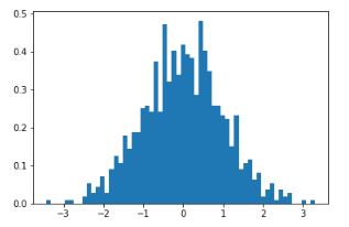
Plot z density (bijectors not applied):

plt.hist(z, bins=60, density=True)
plt.show()

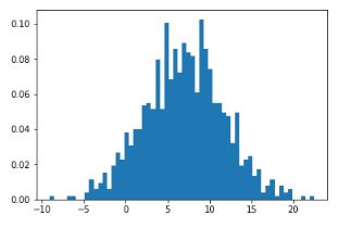
Plot x density (after applying Shift and Scale bijectors):

plt.hist(x, bins=60, density=True)
plt.show()

Inverse Transformation

inv_x = scale_and_shift.inverse(x)

Assert that the inverse transformation is mathematically correct by subtracting the reconstructed inputs (inv_x) from the original inputs (z) to verify the difference is exactly 0.

tf.norm(inv_x - z)

Output:

<tf.Tensor: shape=(), dtype=float32, numpy=0.0>

Log Probability

Log prob of z:

log_prob_z = normal.log_prob(z)

Log prob of x:

\log p_X(x) = \log p_Z(z) – \log \left\vert{} \frac{dx}{dz} \right\vert{}

log_prob_x = normal.log_prob(z) - scale_and_shift.forward_log_det_jacobian(z, event_ndims=0)

We can also use the inverse transformation:

log_prob_x = normal.log_prob(scale_and_shift.inverse(x)) + scale_and_shift.inverse_log_det_jacobian(x, event_ndims=0)

Softfloor Bijector

Create a single bijector with a single temperature:

softfloor_single = tfb.Softfloor(temperature=0.2)

Create a transformed distribution:

transformed_normal_single = tfd.TransformedDistribution(
    distribution=normal,
    bijector=softfloor_single
)

Transform z:

transformed_z_single = softfloor_single.forward(z)

Softfloor Bijector with Broadcasting

Create a batch of bijectors by passing a list of temperatures:

softfloor_batch = tfb.Softfloor(temperature=[0.2, 0.4])

Create a transformed distribution and transform z:

transformed_normal_batch = tfd.TransformedDistribution(
    distribution=normal,
    bijector=softfloor_batch
)
transformed_z_batch = softfloor_batch.forward(z)

MultiVariate Normal

Parameters

A 1D Normal distribution needs two parameters: a mean $(\mu)$ and a variance $(\sigma^2)$ .

When you scale this to multiple dimensions, those scalars become a mean vector $(\boldsymbol{\mu})$ and a covariance matrix $(\boldsymbol{\Sigma})$ .

mu = tf.constant([5.0, 1.0])
covariance_matrix = tf.constant([
    [3.0, 0.5],
    [0.5, 1.5]
])

print("Covariance Matrix:\n", covariance_matrix.numpy())

Cholesky Factor

Cholesky decomposition breaks down a symmetric, positive definite covariance matrix into a lower triangular:

try:
    scale_tril = tf.linalg.cholesky(covariance_matrix)
    print("Cholesky Factor (L):\n", scale_tril.numpy())
except tf.errors.InvalidArgumentError:
    print("Decomposition failed! Matrix is not positive-definite.")

Create the MVN

Use MultivariateNormalTriL with the mean vector and the Cholesky lower triangular matrix:

mvn = tfd.MultivariateNormalTriL(
    loc=mu,
    scale_tril=scale_tril
)

Sampling and Evaluating Densities

samples = mvn.sample(5)
print("Samples:\n", samples.numpy())

likely_point = tf.constant([5.0, 1.0])
unlikely_point = tf.constant([-10.0, -10.0])

print("Likely Log-Prob:   ", mvn.log_prob(likely_point).numpy())
print("Unlikely Log-Prob: ", mvn.log_prob(unlikely_point).numpy())

Subclassing Bijectors

Define a Bijector

class MySigmoid(tfb.Bijector):
    def __init__(self, validate_args=False, name='sigmoid'):
        super(MySigmoid, self).__init__(validate_args=validate_args, forward_min_event_ndims=0, name=name)
        
    def _forward(self, x):
        return tf.math.sigmoid(x)
    
    def _inverse(self, y):
        return tf.math.log(y) - tf.math.log(1 - y)
    
    def _inverse_log_det_jacobian(self, y):
        return -tf.math.log(y) - tf.math.log(1 - y)
    
    def _forward_log_det_jacobian(self, x):
        return -self.inverse_log_det_jacobian(self._forward(x))

You only need to define one of the two log determinant Jacobians:

class Cubic(tfb.Bijector):
    def __init__(self, a, b, validate_args=False, name='Cubic'):
        self.a = tf.cast(a, tf.float32)
        self.b = tf.cast(b, tf.float32)
        
        if validate_args:
            assert tf.reduce_mean(tf.cast(tf.math.greater_equal(tf.abs(self.a), 1e-5), tf.float32)) == 1.0
            assert tf.reduce_mean(tf.cast(tf.math.greater_equal(tf.abs(self.b), 1e-5), tf.float32)) == 1.0
            
        super(Cubic, self).__init__(validate_args=validate_args, forward_min_event_ndims=0, name=name)
        
    def _forward(self, x):
        x = tf.cast(x, tf.float32)
        return tf.squeeze(tf.pow(self.a * x + self.b, 3))
        
    def _inverse(self, y):
        y = tf.cast(y, tf.float32)
        return (tf.math.sign(y) * tf.pow(tf.abs(y), 1/3) - self.b) / self.a
    
    def _forward_log_det_jacobian(self, x):
        x = tf.cast(x, tf.float32)
        return tf.math.log(3. * tf.abs(self.a)) + 2. * tf.math.log(tf.abs(self.a * x + self.b))

Apply Forward Transformation

cubic = Cubic([1., -2.], [-1., 0.4], validate_args=True)

x = tf.constant([[1,2], [3,4]])
y = cubic.forward(x)

Check Inverse

np.linalg.norm(x - cubic.inverse(y))

Output: 0.0

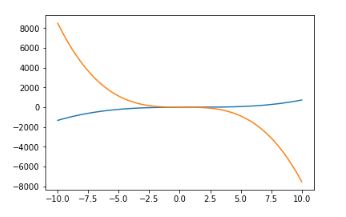
Plot the Forward Transformation

x = np.linspace(-10, 10, 500).reshape(-1, 1)
plt.plot(x, cubic.forward(x))

Plot the Inverse

plt.plot(x, cubic.inverse(x))

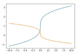
Plot the Forward Log Jacobian Determinant

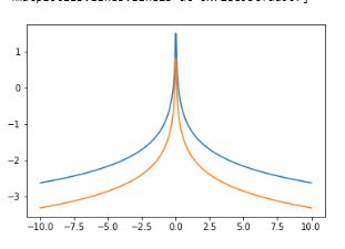
plt.plot(x, cubic.forward_log_det_jacobian(x, event_ndims=0))

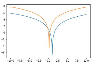
Plot the Inverse Log Jacobian Determinant

plt.plot(x, cubic.inverse_log_det_jacobian(x, event_ndims=0))

Natville